Building a Local Face Search Engine — A Step by Step Guide
Building a Local Face Search Engine — A Step by Step Guide
Part 1: on face embeddings and how to run face search on the fly

In this entry (Part 1) we’ll introduce the basic concepts for face recognition and search, and implement a basic working solution purely in Python. At the end of the article you will be able to run arbitrary face search on the fly, locally on your own images.
In Part 2 we’ll scale the learning of Part 1, by using a vector database to optimize interfacing and querying.
Face matching, embeddings and similarity metrics.
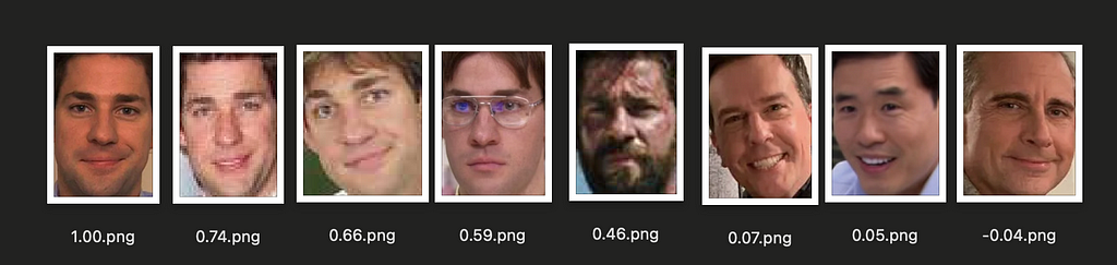
The goal: find all instances of a given query face within a pool of images.
Instead of limiting the search to exact matches only, we can relax the criteria by sorting results based on similarity. The higher the similarity score, the more likely the result to be a match. We can then pick only the top N results or filter by those with a similarity score above a certain threshold.
To sort results, we need a similarity score for each pair of faces <Q, T> (where Q is the query face and T is the target face). While a basic approach might involve a pixel-by-pixel comparison of cropped face images, a more powerful and effective method uses embeddings.
An embedding is a learned representation of some input in the form of a list of real-value numbers (a N-dimensional vector). This vector should capture the most essential features of the input, while ignoring superfluous aspect; an embedding is a distilled and compacted representation.
Machine-learning models are trained to learn such representations and can then generate embeddings for newly seen inputs. Quality and usefulness of embeddings for a use-case hinge on the quality of the embedding model, and the criteria used to train it.
In our case, we want a model that has been trained to maximize face identity matching: photos of the same person should match and have very close representations, while the more faces identities differ, the more different (or distant) the related embeddings should be. We want irrelevant details such as lighting, face orientation, face expression to be ignored.
Once we have embeddings, we can compare them using well-known distance metrics like cosine similarity or Euclidean distance. These metrics measure how “close” two vectors are in the vector space. If the vector space is well structured (i.e., the embedding model is effective), this will be equivalent to know how similar two faces are. With this we can then sort all results and select the most likely matches.
https://medium.com/media/8929d6d8077c7300dfa5acc29dba739b/href
Implement and Run Face Search
Let’s jump on the implementation of our local face search. As a requirement you will need a Python environment (version ≥3.10) and a basic understanding on the Python language.
For our use-case we will also rely on the popular Insightface library, which on top of many face-related utilities, also offers face embeddings (aka recognition) models. This library choice is just to simplify the process, as it takes care of downloading, initializing and running the necessary models. You can also go directly for the provided ONNX models, for which you’ll have to write some boilerplate/wrapper code.
First step is to install the required libraries (we advise to use a virtual environment).
pip install numpy==1.26.4 pillow==10.4.0 insightface==0.7.3
The following is the script you can use to run a face search. We commented all relevant bits. It can be run in the command-line by passing the required arguments. For example
python run_face_search.py -q "./query.png" -t "./face_search"
https://medium.com/media/bcb2ba4a20ed239be8ffbfa61be89259/href
The query arg should point to the image containing the query face, while the target arg should point to the directory containing the images to search from. Additionally, you can control the similarity-threshold to account for a match, and the minimum resolution required for a face to be considered.
The script loads the query face, computes its embedding and then proceeds to load all images in the target directory and compute embeddings for all found faces. Cosine similarity is then used to compare each found face with the query face. A match is recorded if the similarity score is greater than the provided threshold. At the end the list of matches is printed, each with the original image path, the similarity score and the location of the face in the image (that is, the face bounding box coordinates). You can edit this script to process such output as needed.
Similarity values (and so the threshold) will be very dependent on the embeddings used and nature of the data. In our case, for example, many correct matches can be found around the 0.5 similarity value. One will always need to compromise between precision (match returned are correct; increases with higher threshold) and recall (all expected matches are returned; increases with lower threshold).
What’s Next?
And that’s it! That’s all you need to run a basic face search locally. It is quite accurate, and can be run on the fly, but it doesn’t provide optimal performances. Searching from a large set of images will be slow and, more important, all embeddings will be recomputed for every query. In the next post we will improve on this setup and scale the approach by using a vector database.
Want to Connect?
You can catch a glimpse of my latest experiments and explanations on Twitter or Threads and see my graphics results on Instagram.
Building a Local Face Search Engine — A Step by Step Guide was originally published in Becoming Human: Artificial Intelligence Magazine on Medium, where people are continuing the conversation by highlighting and responding to this story.
LLNL Scientists Use Machine Learning to Probe Carbon Capture at Atomic Level
Unlocking the Power of Hugging Face for NLP Tasks

The field of Natural Language Processing (NLP) has seen significant advancements in recent years, largely driven by the development of sophisticated models capable of understanding and generating human language. One of the key players in this revolution is Hugging Face, an open-source AI company that provides state-of-the-art models for a wide range of NLP tasks. Hugging Face’s Transformers library has become the go-to resource for developers and researchers looking to implement powerful NLP solutions.
Inbound-leads-automatically-with-ai. These models are trained on vast amounts of data and fine-tuned to achieve exceptional performance on specific tasks. The platform also provides tools and resources to help users fine-tune these models on their own datasets, making it highly versatile and user-friendly.
In this blog, we’ll delve into how to use the Hugging Face library to perform several NLP tasks. We’ll explore how to set up the environment, and then walk through examples of sentiment analysis, zero-shot classification, text generation, summarization, and translation. By the end of this blog, you’ll have a solid understanding of how to leverage Hugging Face models to tackle various NLP challenges.
Setting Up the Environment
First, we need to install the Hugging Face Transformers library, which provides access to a wide range of pre-trained models. You can install it using the following command:
!pip install transformers
This library simplifies the process of working with advanced NLP models, allowing you to focus on building your application rather than dealing with the complexities of model training and optimization.
Task 1: Sentiment Analysis
Sentiment analysis determines the emotional tone behind a body of text, identifying it as positive, negative, or neutral. Here’s how it’s done using Hugging Face:
from transformers import pipeline
classifier = pipeline("sentiment-analysis", token = access_token, model='distilbert-base-uncased-finetuned-sst-2-english')
classifier("This is by far the best product I have ever used; it exceeded all my expectations.")
In this example, we use the sentiment-analysis pipeline to classify the sentiments of sentences, determining whether they are positive or negative.


Task 2: Zero-Shot Classification
Zero-shot classification allows the model to classify text into categories without any prior training on those specific categories. Here’s an example:
classifier = pipeline("zero-shot-classification")
classifier(
    "Photosynthesis is the process by which green plants use sunlight to synthesize nutrients from carbon dioxide and water.",
    candidate_labels=["education", "science", "business"],
)
The zero-shot-classification pipeline classifies the given text into one of the provided labels. In this case, it correctly identifies the text as being related to “science”.

Task 3: Text Generation
In this task, we explore text generation using a pre-trained model. The code snippet below demonstrates how to generate text using the GPT-2 model:
generator = pipeline("text-generation", model="distilgpt2")
generator(
"Just finished an amazing book",
max_length=40, num_return_sequences=2,
)
Here, we use the pipeline function to create a text generation pipeline with the distilgpt2 model. We provide a prompt (“Just finished an amazing book”) and specify the maximum length of the generated text. The result is a continuation of the provided prompt.

Task 4: Text Summarization
Next, we use Hugging Face to summarize a long text. The following code shows how to summarize a piece of text using the BART model:
summarizer = pipeline("summarization")
text = """
San Francisco, officially the City and County of San Francisco, is a commercial and cultural center in the northern region of the U.S. state of California. San Francisco is the fourth most populous city in California and the 17th most populous in the United States, with 808,437 residents as of 2022.
"""
summary = summarizer(text, max_length=50, min_length=25, do_sample=False)
print(summary)
The summarization pipeline is used here, and we pass a lengthy piece of text about San Francisco. The model returns a concise summary of the input text.

Task 5: Translation
In the final task, we demonstrate how to translate text from one language to another. The code snippet below shows how to translate French text to English using the Helsinki-NLP model:
translator = pipeline("translation", model="Helsinki-NLP/opus-mt-fr-en")
translation = translator("L'engagement de l'entreprise envers l'innovation et l'excellence est véritablement inspirant.")
print(translation)
Here, we use the translation pipeline with the Helsinki-NLP/opus-mt-fr-en model. The French input text is translated into English, showcasing the model’s ability to understand and translate between languages.

Conclusion
The Hugging Face library offers powerful tools for a variety of NLP tasks. By using simple pipelines, we can perform sentiment analysis, zero-shot classification, text generation, summarization, and translation with just a few lines of code. This notebook serves as an excellent starting point for exploring the capabilities of Hugging Face models in NLP projects.
Feel free to experiment with different models and tasks to see the full potential of Hugging Face in action!
This brings us to the end of this article. I hope you have understood everything clearly. Make sure you practice as much as possible.
If you wish to check out more resources related to Data Science, Machine Learning, and Deep Learning, you can refer to my GitHub account.
You can connect with me on LinkedIn — Ravjot Singh.
P.S. Claps and follows are highly appreciated.
Unlocking the Power of Hugging Face for NLP Tasks was originally published in Becoming Human: Artificial Intelligence Magazine on Medium, where people are continuing the conversation by highlighting and responding to this story.
Comparing ANN and CNN on CIFAR-10: A Comprehensive Analysis
Are you curious about how different neural networks stack up against each other? In this blog, we dive into an exciting comparison between Artificial Neural Networks (ANN) and Convolutional Neural Networks (CNN) using the popular CIFAR-10 dataset. We’ll break down the key concepts, architectural differences, and real-world applications of ANNs and CNNs. Join us as we uncover which model reigns supreme for image classification tasks and why. Let’s get started!
Dataset Overview
The CIFAR-10 dataset is a widely-used dataset for machine learning and computer vision tasks. It consists of 60,000 32×32 color images in 10 different classes, with 50,000 training images and 10,000 test images. The classes are airplanes, cars, birds, cats, deer, dogs, frogs, horses, ships, and trucks. This blog explores the performance of Artificial Neural Networks (ANN) and Convolutional Neural Networks (CNN) on the CIFAR-10 dataset.

What is ANN?
Artificial Neural Networks (ANN) are computational models inspired by the human brain. They consist of interconnected groups of artificial neurons (nodes) that process information using a connectionist approach. ANNs are used for a variety of tasks, including classification, regression, and pattern recognition.
Principles of ANN
- Layers: ANNs consist of input, hidden, and output layers.
- Neurons: Each layer has multiple neurons that process inputs and produce outputs.
- Activation Functions: Functions like ReLU or Sigmoid introduce non-linearity, enabling the network to learn complex patterns.
- Backpropagation: The learning process involves adjusting weights based on the error gradient.

ANN Architecture
ANN = models.Sequential([
    layers.Flatten(input_shape=(32, 32, 3)),
    layers.Dense(3000, activation='relu'),
    layers.Dense(1000, activation='relu'),
    layers.Dense(10, activation='sigmoid')
])
ANN.compile(optimizer='adam', loss='sparse_categorical_crossentropy', metrics=['accuracy'
What is CNN?
Convolutional Neural Networks (CNN) are specialized ANNs designed for processing structured grid data, like images. They are particularly effective for tasks involving spatial hierarchies, such as image classification and object detection.
Principles of CNN
- Convolutional Layers: These layers apply convolutional filters to the input to extract features.
- Pooling Layers: Pooling layers reduce the spatial dimensions, retaining important information while reducing computational load.
- Fully Connected Layers: After convolutional and pooling layers, fully connected layers are used to make final predictions.

CNN Architecture
CNN = models.Sequential([
    layers.Conv2D(input_shape=(32, 32, 3), filters=32, kernel_size=(3, 3), activation='relu'),
    layers.MaxPooling2D((2, 2)),
    layers.Conv2D(filters=64, kernel_size=(3, 3), activation='relu'),
    layers.MaxPooling2D((2, 2)),
    layers.Flatten(),
    layers.Dense(2000, activation='relu'),
    layers.Dense(1000, activation='relu'),
    layers.Dense(10, activation='softmax')
])
CNN.compile(optimizer='adam', loss='sparse_categorical_crossentropy', metrics=['accuracy'])
Training and Evaluation
Both models were trained for 10 epochs on the CIFAR-10 dataset. The ANN model uses dense layers and is simpler, while the CNN model uses convolutional and pooling layers, making it more complex and suitable for image data.
ANN.fit(X_train, y_train, epochs=10)
ANN.evaluate(X_test, y_test)

CNN.fit(X_train, y_train, epochs=10)
CNN.evaluate(X_test, y_test)


Results Comparison
The evaluation results for both models show the accuracy and loss on the test data.
ANN Evaluation
- Accuracy: 0.4960
- Loss: 1.4678

CNN Evaluation
- Accuracy: 0.7032
- Loss: 0.8321

The CNN significantly outperforms the ANN in terms of accuracy and loss.
Confusion Matrices and Classification Reports
To further analyze the models’ performance, confusion matrices and classification reports were generated.
ANN Confusion Matrix and Report
y_pred_ann = ANN.predict(X_test)
y_pred_labels_ann = [np.argmax(i) for i in y_pred_ann]
plot_confusion_matrix(y_test, y_pred_labels_ann, "Confusion Matrix for ANN")
print("Classification Report for ANN:")
print(classification_report(y_test, y_pred_labels_ann))

CNN Confusion Matrix and Report
y_pred_cnn = CNN.predict(X_test)
y_pred_labels_cnn = [np.argmax(i) for i in y_pred_cnn]
plot_confusion_matrix(y_test, y_pred_labels_cnn, "Confusion Matrix for CNN")
print("Classification Report for CNN:")
print(classification_report(y_test, y_pred_labels_cnn))

Conclusion
The CNN model outperforms the ANN model on the CIFAR-10 dataset due to its ability to capture spatial hierarchies and local patterns in the image data. While ANNs are powerful for general tasks, CNNs are specifically designed for image-related tasks, making them more effective for this application.
In summary, for image classification tasks like those in the CIFAR-10 dataset, CNNs offer a significant performance advantage over ANNs due to their specialized architecture tailored for processing visual data.
This brings us to the end of this article. I hope you have understood everything clearly. Make sure you practice as much as possible.
If you wish to check out more resources related to Data Science, Machine Learning and Deep Learning you can refer to my Github account.
You can connect with me on LinkedIn — RAVJOT SINGH.
P.S. Claps and follows are highly appreciated.
Comparing ANN and CNN on CIFAR-10: A Comprehensive Analysis was originally published in Becoming Human: Artificial Intelligence Magazine on Medium, where people are continuing the conversation by highlighting and responding to this story.
Exploring NLP Preprocessing Techniques: Stopwords, Bag of Words, and Word Cloud
Natural Language Processing (NLP) is a fascinating field that bridges the gap between human communication and machine understanding. One of the fundamental steps in NLP is text preprocessing, which transforms raw text data into a format that can be effectively analyzed and utilized by algorithms. In this blog, we’ll delve into three essential NLP preprocessing techniques: stopwords removal, bag of words, and word cloud generation. We’ll explore what each technique is, why it’s used, and how to implement it using Python. Let’s get started!
Stopwords Removal: Filtering Out the Noise
What Are Stopwords?
Stopwords are common words that carry little meaningful information and are often removed from text data during preprocessing. Examples include “the,” “is,” “in,” “and,” etc. Removing stopwords helps in focusing on the more significant words that contribute to the meaning of the text.
Why remove stopwords?
Stopwords are removed from:
- Reduce the dimensionality of the text data.
- Improve the efficiency and performance of NLP models.
- Enhance the relevance of features extracted from the text.
Pros and Cons
Pros:
- Simplifies the text data.
- Reduces computational complexity.
- Focuses on meaningful words.
Cons:
- Risk of removing words that may carry context-specific importance.
- Some NLP tasks may require stopwords for better understanding.
Implementation
Let’s see how we can remove stopwords using Python:
import nltk
from nltk.corpus import stopwords
# Download the stopwords dataset
nltk.download('stopwords')
# Sample text
text = "This is a simple example to demonstrate stopword removal in NLP."
Load the set of stopwords in English
stop_words = set(stopwords.words('english'))
Tokenize the text into individual words
words = text.split()
Remove stopwords from the text
filtered_text = [word for word in words if word.lower() is not in stop_words]
print("Original Text:", text)
print("Filtered Text:", " ".join(filtered_text))
Code Explanation
Importing Libraries:
import nltk from nltk.corpus import stopwords
We import thenltk library and the stopwords module fromnltk.corpus.
Downloading Stopwords:
nltk.download('stopwords')
This line downloads the stopwords dataset from the NLTK library, which includes a list of common stopwords for multiple languages.
Sample Text:
text = "This is a simple example to demonstrate stopword removal in NLP."
We define a sample text that we want to preprocess by removing stopwords.
Loading Stopwords:
stop_words = set(stopwords.words(‘english’))
We load the set of English stopwords into the variable stop_words.
Tokenizing Text:
words = text.split()
The split() method tokenizes the text into individual words.
Removing Stopwords:
filtered_text = [word for word in words if word.lower() is not in stop_words]
We use a list comprehension to filter out stopwords from the tokenized words. The lower() method ensures case insensitivity.
Printing Results:
print("Original Text:", text) print("Filtered Text:", ""). join(filtered_text))
Finally, we print the original text and the filtered text after removing stopwords.
Bag of Words: Representing Text Data as Vectors
What Is Bag of Words?
The Bag of Words (BoW) model is a technique to represent text data as vectors of word frequencies. Each document is represented as a vector where each dimension corresponds to a unique word in the corpus, and the value indicates the word’s frequency in the document.
Why Use Bag of Words?
bag of Words is used to:
- Convert text data into numerical format for machine learning algorithms.
- Capture the frequency of words, which can be useful for text classification and clustering tasks.
Pros and Cons
Pros:
- Simple and easy to implement.
- Effective for many text classification tasks.
Cons:
- Ignores word order and context.
- Can result in high-dimensional sparse vectors.
Implementation
Here’s how to implement the Bag of Words model using Python:
from sklearn.feature_extraction.text import CountVectorizer
# Sample documents
documents = [
    'This is the first document',
    'This document is the second document',
    'And this is the third document.',
    'Is this the first document?'
]
# Initialize CountVectorizer
vectorizer = CountVectorizer()
Fit and transform the documents
X = vectorizer.fit_transform(documents)
# Convert the result to an array
X_array = X.toarray()
# Get the feature names
feature_names = vectorizer.get_feature_names_out()
# Print the feature names and the Bag of Words representation
print("Feature Names:", feature_names)
print (Bag of Words: n", X_array)
Code Explanation
- Importing Libraries:
from sklearn.feature_extraction.text import CountVectorizer
We import the CountVectorizer from the sklearn.feature_extraction.text module.
Sample Documents:
documents = [ ‘This is the first document’, ‘This document is the second document’, ‘And this is the third document.’, ‘Is this is the first document?’ ]
We define a list of sample documents to be processed.
Initializing CountVectorizer:
vectorizer = CountVectorizer()
We create an instance ofCountVectorizer.
Fitting and Transforming:
X = vectorizer.fit_transform(documents)
Thefit_transform method is used to fit the model and transform the documents into a bag of words.
Converting to an array:
X_array = X.toarray()
We convert the sparse matrix result to a dense array for easy viewing.
Getting Feature Names:
feature_names = vectorizer.get_feature_names_out()
The get_feature_names_out method retrieves the unique words identified in the corpus.
Printing Results:
print(“Feature Names:”, feature_names) print(“Bag of Words: n”, X_array)

Finally, we print the feature names and the bag of words.
Word Cloud: Visualizing Text Data
What Is a Word Cloud?
A word cloud is a visual representation of text data where the size of each word indicates its frequency or importance. It provides an intuitive and appealing way to understand the most prominent words in a text corpus.
Why Use Word Cloud?
Word clouds are used to:
- Quickly grasp the most frequent terms in a text.
- Visually highlight important keywords.
- Present text data in a more engaging format.
Pros and Cons
Pros:
- Easy to interpret and visually appealing.
- Highlights key terms effectively.
Cons:
- Can oversimplify the text data.
- May not be suitable for detailed analysis.
Implementation
Here’s how to create a word cloud using Python:
from wordcloud import WordCloud
import matplotlib.pyplot as plt
# Sample text
df = pd.read_csv('/content/AmazonReview.csv')
comment_words = ""
stopwords = set(STOPWORDS)
for val in df.Review:
     val = str(val)
     tokens = val.split()
     for i in range(len(tokens)):
     tokens[i] = tokens[i].lower()
     comment_words += "".join(tokens) + ""
pic = np.array(Image.open(requests.get('https://www.clker.com/cliparts/a/c/3/6/11949855611947336549home14.svg.med.png', stream = True).raw))
# Generate word clouds
wordcloud = WordCloud(width=800, height=800, background_color='white', mask=pic, min_font_size=12).generate(comment_words)
Display the word cloud
plt.figure(figsize=(8,8), facecolor=None)
plt.imshow(wordcloud)
plt.axis('off')
plt.tight_layout(pad=0)
plt.show()
Code Explanation
- Importing Libraries:
from wordcloud import WordCloud import matplotlib.pyplot as plt
We import the WordCloud class from the wordcloud library and matplotlib.pyplot for displaying the word cloud.
Generating Word Clouds:
wordcloud = WordCloud(width=800, height=800, background_color=’white’).generate(comment_words)
We create an instance of WordCloud with specified dimensions and background color and generate the word cloud using the sample text.

Conclusion
In this blog, we’ve explored three essential NLP preprocessing techniques: stopwords removal, bag of words, and word cloud generation. Each technique serves a unique purpose in the text preprocessing pipeline, contributing to the overall effectiveness of NLP tasks. By understanding and implementing these techniques, we can transform raw text data into meaningful insights and powerful features for machine learning models. Happy coding and exploring the world of NLP!
This brings us to the end of this article. I hope you have understood everything clearly. Make sure you practice as much as possible.
If you wish to check out more resources related to Data Science, Machine Learning and Deep learning, you can refer to my Github account.
You can connect with me on LinkedIn — RAVJOT SINGH.
I hope you like my article. From a future perspective, you can try other algorithms or choose different values of parameters to improve the accuracy even further. Please feel free to share your thoughts and ideas.
P.S. Claps and follows are highly appreciated.
Exploring NLP Preprocessing Techniques: Stopwords, Bag of Words, and Word Cloud was originally published in Becoming Human: Artificial Intelligence Magazine on Medium, where people are continuing the conversation by highlighting and responding to this story.
Machine Learning Revolutionizes Flood Relief Efforts in Assam
Unveiling Machine Learning Algorithms Behind AI Chatbots
Understanding Tokenization, Stemming, and Lemmatization in NLP
Natural Language Processing (NLP) involves various techniques to handle and analyze human language data. In this blog, we will explore three essential techniques: tokenization, stemming, and lemmatization. These techniques are foundational for many NLP applications, such as text preprocessing, sentiment analysis, and machine translation. Let’s delve into each technique, understand its purpose, pros and cons, and see how they can be implemented using Python’s NLTK library.

1. Tokenization
What is Tokenization?
Tokenization is the process of splitting a text into individual units, called tokens. These tokens can be words, sentences, or subwords. Tokenization helps break down complex text into manageable pieces for further processing and analysis.
Why is Tokenization Used?
Tokenization is the first step in text preprocessing. It transforms raw text into a format that can be analyzed. This process is essential for tasks such as text mining, information retrieval, and text classification.
Pros and Cons of Tokenization
Pros:
- Simplifies text processing by breaking text into smaller units.
- Facilitates further text analysis and NLP tasks.
Cons:
- Can be complex for languages without clear word boundaries.
- May not handle special characters and punctuation well.
Code Implementation
Here is an example of tokenization using the NLTK library:
# Install NLTK library
!pip install nltk
Explanation:
- !pip install nltk: This command installs the NLTK library, which is a powerful toolkit for NLP in Python.
# Sample text
tweet = "Sometimes to understand a word's meaning you need more than a definition. you need to see the word used in a sentence."
Explanation:
- tweet: This is a sample text we will use for tokenization. It contains multiple sentences and words.
# Importing required modules
import nltk
nltk.download('punkt')
Explanation:
- import nltk: This imports the NLTK library.
- nltk.download(‘punkt’): This downloads the ‘punkt’ tokenizer models, which are necessary for tokenization.
from nltk.tokenize import word_tokenize, sent_tokenize
Explanation:
- from nltk.tokenize import word_tokenize, sent_tokenize: This imports the word_tokenize and sent_tokenize functions from the NLTK library for word and sentence tokenization, respectively.
# Word Tokenization
text = "Hello! how are you?"
word_tok = word_tokenize(text)
print(word_tok)
Explanation:
- text: This is a simple sentence we will tokenize into words.
- word_tok = word_tokenize(text): This tokenizes the text into individual words.
- print(word_tok): This prints the list of word tokens. Output: [‘Hello’, ‘!’, ‘how’, ‘are’, ‘you’, ‘?’]
# Sentence Tokenization
sent_tok = sent_tokenize(tweet)
print(sent_tok)
Explanation:
- sent_tok = sent_tokenize(tweet): This tokenizes the tweet into individual sentences.
- print(sent_tok): This prints the list of sentence tokens. Output: [‘Sometimes to understand a word’s meaning you need more than a definition.’, ‘you need to see the word used in a sentence.’]
2. Stemming
What is Stemming?
Stemming is the process of reducing a word to its base or root form. It involves removing suffixes and prefixes from words to derive the stem.
Why is Stemming Used?
Stemming helps in normalizing words to their root form, which is useful in text mining and search engines. It reduces inflectional forms and derivationally related forms of a word to a common base form.
Pros and Cons of Stemming
Pros:
- Reduces the complexity of text by normalizing words.
- Improves the performance of search engines and information retrieval systems.
Cons:
- Can lead to incorrect base forms (e.g., ‘running’ to ‘run’, but ‘flying’ to ‘fli’).
- Different stemming algorithms may produce different results.
Code Implementation
Let’s see how to perform stemming using different algorithms:
Porter Stemmer:
from nltk.stem import PorterStemmer
stemming = PorterStemmer()
word = 'danced'
print(stemming.stem(word))
Explanation:
- from nltk.stem import PorterStemmer: This imports the PorterStemmer class from NLTK.
- stemming = PorterStemmer(): This creates an instance of the PorterStemmer.
- word = ‘danced’: This is the word we want to stem.
- print(stemming.stem(word)): This prints the stemmed form of the word ‘danced’. Output: danc
word = 'replacement'
print(stemming.stem(word))
Explanation:
- word = ‘replacement’: This is another word we want to stem.
- print(stemming.stem(word)): This prints the stemmed form of the word ‘replacement’. Output: replac
word = 'happiness'
print(stemming.stem(word))
Explanation:
- word = ‘happiness’: This is another word we want to stem.
- print(stemming.stem(word)): This prints the stemmed form of the word ‘happiness’. Output: happi
Lancaster Stemmer:
from nltk.stem import LancasterStemmer
stemming1 = LancasterStemmer()
word = 'happily'
print(stemming1.stem(word))
Explanation:
- from nltk.stem import LancasterStemmer: This imports the LancasterStemmer class from NLTK.
- stemming1 = LancasterStemmer(): This creates an instance of the LancasterStemmer.
- word = ‘happily’: This is the word we want to stem.
- print(stemming1.stem(word)): This prints the stemmed form of the word ‘happily’. Output: happy
Regular Expression Stemmer:
from nltk.stem import RegexpStemmer
stemming2 = RegexpStemmer('ing$|s$|e$|able$|ness$', min=3)
word = 'raining'
print(stemming2.stem(word))
Explanation:
- from nltk.stem import RegexpStemmer: This imports the RegexpStemmer class from NLTK.
- stemming2 = RegexpStemmer(‘ing$|s$|e$|able$|ness$’, min=3): This creates an instance of the RegexpStemmer with a regular expression pattern to match suffixes and a minimum stem length of 3 characters.
- word = ‘raining’: This is the word we want to stem.
- print(stemming2.stem(word)): This prints the stemmed form of the word ‘raining’. Output: rain
word = 'flying'
print(stemming2.stem(word))
Explanation:
- word = ‘flying’: This is another word we want to stem.
- print(stemming2.stem(word)): This prints the stemmed form of the word ‘flying’. Output: fly
word = 'happiness'
print(stemming2.stem(word))
Explanation:
- word = ‘happiness’: This is another word we want to stem.
- print(stemming2.stem(word)): This prints the stemmed form of the word ‘happiness’. Output: happy
Snowball Stemmer:
nltk.download("snowball_data")
from nltk.stem import SnowballStemmer
stemming3 = SnowballStemmer("english")
word = 'happiness'
print(stemming3.stem(word))
Explanation:
- nltk.download(“snowball_data”): This downloads the Snowball stemmer data.
- from nltk.stem import SnowballStemmer: This imports the SnowballStemmer class from NLTK.
- stemming3 = SnowballStemmer(“english”): This creates an instance of the SnowballStemmer for the English language.
- word = ‘happiness’: This is the word we want to stem.
- print(stemming3.stem(word)): This prints the stemmed form of the word ‘happiness’. Output: happy
stemming3 = SnowballStemmer("arabic")
word = 'تحلق'
print(stemming3.stem(word))
Explanation:
- stemming3 = SnowballStemmer(“arabic”): This creates an instance of the SnowballStemmer for the Arabic language.
- word = ‘تحلق’: This is an Arabic word we want to stem.
- print(stemming3.stem(word)): This prints the stemmed form of the word ‘تحلق’. Output: تحل
3. Lemmatization
What is Lemmatization?
Lemmatization is the process of reducing a word to its base or dictionary form, known as a lemma. Unlike stemming, lemmatization considers the context and converts the word to its meaningful base form.
Why is Lemmatization Used?
Lemmatization provides more accurate base forms compared to stemming. It is widely used in text analysis, chatbots, and NLP applications where understanding the context of words is essential.
Pros and Cons of Lemmatization
Pros:
- Produces more accurate base forms by considering the context.
- Useful for tasks requiring semantic understanding.
Cons:
- Requires more computational resources compared to stemming.
- Dependent on language-specific dictionaries.
Code Implementation
Here is how to perform lemmatization using the NLTK library:
# Download necessary data
nltk.download('wordnet')
Explanation:
- nltk.download(‘wordnet’): This command downloads the WordNet corpus, which is used by the WordNetLemmatizer for finding the lemmas of words.
from nltk.stem import WordNetLemmatizer
lemmatizer = WordNetLemmatizer()
Explanation:
- from nltk.stem import WordNetLemmatizer: This imports the WordNetLemmatizer class from NLTK.
- lemmatizer = WordNetLemmatizer(): This creates an instance of the WordNetLemmatizer.
print(lemmatizer.lemmatize('going', pos='v'))
Explanation:
- lemmatizer.lemmatize(‘going’, pos=’v’): This lemmatizes the word ‘going’ with the part of speech (POS) tag ‘v’ (verb). Output: go
# Lemmatizing a list of words with their respective POS tags
words = [("eating", 'v'), ("playing", 'v')]
for word, pos in words:
    print(lemmatizer.lemmatize(word, pos=pos))
Explanation:
- words = [(“eating”, ‘v’), (“playing”, ‘v’)]: This is a list of tuples where each tuple contains a word and its corresponding POS tag.
- for word, pos in words: This iterates through each tuple in the list.
- print(lemmatizer.lemmatize(word, pos=pos)): This prints the lemmatized form of each word based on its POS tag. Outputs: eat, play
Applications in NLP
- Tokenization is used in text preprocessing, sentiment analysis, and language modeling.
- Stemming is useful for search engines, information retrieval, and text mining.
- Lemmatization is essential for chatbots, text classification, and semantic analysis.
Conclusion
Tokenization, stemming, and lemmatization are crucial techniques in NLP. They transform the raw text into a format suitable for analysis and help in understanding the structure and meaning of the text. By applying these techniques, we can enhance the performance of various NLP applications.
Feel free to experiment with the provided code snippets and explore these techniques further. Happy coding!
This brings us to the end of this article. I hope you have understood everything clearly. Make sure you practice as much as possible.
If you wish to check out more resources related to Data Science, Machine Learning and Deep Learning you can refer to my Github account.
You can connect with me on LinkedIn — RAVJOT SINGH.
I hope you like my article. From a future perspective, you can try other algorithms also, or choose different values of parameters to improve the accuracy even further. Please feel free to share your thoughts and ideas.
P.S. Claps and follows are highly appreciated.
Understanding Tokenization, Stemming, and Lemmatization in NLP was originally published in Becoming Human: Artificial Intelligence Magazine on Medium, where people are continuing the conversation by highlighting and responding to this story.
Building Your First Deep Learning Model: A Step-by-Step Guide
Introduction to Deep Learning
Deep learning is a subset of machine learning, which itself is a subset of artificial intelligence (AI). Deep learning models are inspired by the structure and function of the human brain and are composed of layers of artificial neurons. These models are capable of learning complex patterns in data through a process called training, where the model is iteratively adjusted to minimize errors in its predictions.
In this blog post, we will walk through the process of building a simple artificial neural network (ANN) to classify handwritten digits using the MNIST dataset.

Understanding the MNIST Dataset
The MNIST dataset (Modified National Institute of Standards and Technology dataset) is one of the most famous datasets in the field of machine learning and computer vision. It consists of 70,000 grayscale images of handwritten digits from 0 to 9, each of size 28×28 pixels. The dataset is divided into a training set of 60,000 images and a test set of 10,000 images. Each image is labeled with the corresponding digit it represents.
Downloading the Dataset
We will use the MNIST dataset provided by the Keras library, which makes it easy to download and use in our model.
Step 1: Importing the Required Libraries
Before we start building our model, we need to import the necessary libraries. These include libraries for data manipulation, visualization, and building our deep learning model.
import numpy as np
import pandas as pd
import matplotlib.pyplot as plt
import seaborn as sns
import tensorflow as tf
from tensorflow import keras
- numpy and pandas are used for numerical and data manipulation.
- matplotlib and seaborn are used for data visualization.
- tensorflow and keras are used for building and training the deep learning model.
Step 2: Loading the Dataset
The MNIST dataset is available directly in the Keras library, making it easy to load and use.
(X_train, y_train), (X_test, y_test) = keras.datasets.mnist.load_data()
This line of code downloads the MNIST dataset and splits it into training and test sets:
- X_train and y_train are the training images and their corresponding labels.
- X_test and y_test are the test images and their corresponding labels.
Step 3: Inspecting the Dataset
Let’s take a look at the shape of our training and test datasets to understand their structure.
print(X_train.shape)
print(X_test.shape)
print(y_train.shape)
print(y_test.shape)
- X_train.shape outputs (60000, 28, 28), indicating there are 60,000 training images, each of size 28×28 pixels.
- X_test.shape outputs (10000, 28, 28), indicating there are 10,000 test images, each of size 28×28 pixels.
- y_train.shape outputs (60000,), indicating there are 60,000 training labels.
- `y_test
.shapeoutputs(10000,)`, indicating there are 10,000 test labels.
To get a better understanding, let’s visualize one of the training images and its corresponding label.
plt.imshow(X_train[2], cmap='gray')
plt.show()
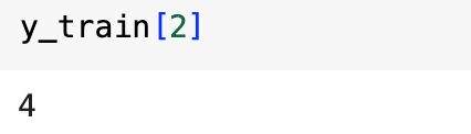
print(y_train[2])
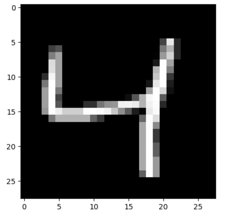
- plt.imshow(X_train[2], cmap=’gray’) displays the third image in the training set in grayscale.
- plt.show() renders the image.
- print(y_train[2]) outputs the label for the third image, which is the digit the image represents.
Step 4: Rescaling the Dataset
Pixel values in the images range from 0 to 255. To improve the performance of our neural network, we rescale these values to the range [0, 1].
X_train = X_train / 255
X_test = X_test / 255
This normalization helps the neural network learn more efficiently by ensuring that the input values are in a similar range.
Step 5: Reshaping the Dataset
Our neural network expects the input to be a flat vector rather than a 2D image. Therefore, we reshape our training and test datasets accordingly.
X_train = X_train.reshape(len(X_train), 28 * 28)
X_test = X_test.reshape(len(X_test), 28 * 28)
- X_train.reshape(len(X_train), 28 * 28) reshapes the training set from (60000, 28, 28) to (60000, 784), flattening each 28×28 image into a 784-dimensional vector.
- Similarly, X_test.reshape(len(X_test), 28 * 28) reshapes the test set from (10000, 28, 28) to (10000, 784).
Step 6: Building Our First ANN Model
We will build a simple neural network with one input layer and one output layer. The input layer will have 784 neurons (one for each pixel), and the output layer will have 10 neurons (one for each digit).
ANN1 = keras.Sequential([
    keras.layers.Dense(10, input_shape=(784,), activation='sigmoid')
])
- keras.Sequential() creates a sequential model, which is a linear stack of layers.
- keras.layers.Dense(10, input_shape=(784,), activation=’sigmoid’) adds a dense (fully connected) layer with 10 neurons, input shape of 784, and sigmoid activation function.
Next, we compile our model by specifying the optimizer, loss function, and metrics.
ANN1.compile(optimizer='adam', loss='sparse_categorical_crossentropy', metrics=['accuracy'])
- optimizer=’adam’ specifies the Adam optimizer, which is an adaptive learning rate optimization algorithm.
- loss=’sparse_categorical_crossentropy’ specifies the loss function, which is suitable for multi-class classification problems.
- metrics=[‘accuracy’] specifies that we want to track accuracy during training.
We then train the model on the training data.
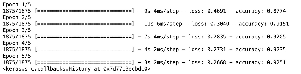
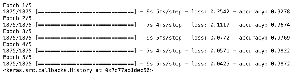
ANN1.fit(X_train, y_train, epochs=5)
- ANN1.fit(X_train, y_train, epochs=5) trains the model for 5 epochs. An epoch is one complete pass through the training data.
Step 7: Evaluating the Model
After training the model, we evaluate its performance on the test data.
ANN1.evaluate(X_test, y_test)
- ANN1.evaluate(X_test, y_test) evaluates the model on the test data and returns the loss value and metrics specified during compilation.

Step 8: Making Predictions
We can use our trained model to make predictions on the test data.
y_predicted = ANN1.predict(X_test)
- ANN1.predict(X_test) generates predictions for the test images.

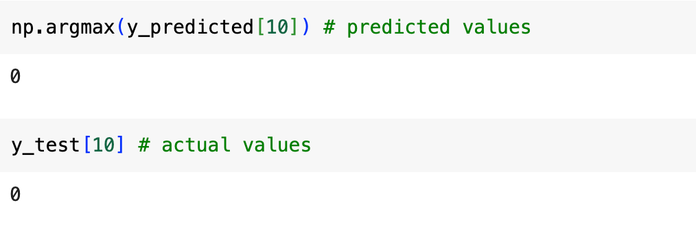
To see the predicted label for the first test image:
print(np.argmax(y_predicted[10]))
print(y_test[10])
- np.argmax(y_predicted[10]) returns the index of the highest value in the prediction vector, which corresponds to the predicted digit.
- print(y_test[10]) prints the actual label of the first test image for comparison.
Step 9: Building a More Complex ANN Model
To improve our model, we add a hidden layer with 150 neurons and use the ReLU activation function, which often performs better in deep learning models.
ANN2 = keras.Sequential([
    keras.layers.Dense(150, input_shape=(784,), activation='relu'),
    keras.layers.Dense(10, activation='sigmoid')
])
- keras.layers.Dense(150, input_shape=(784,), activation=’relu’) adds a dense hidden layer with 150 neurons and ReLU activation function.
We compile and train the improved model in the same way.
ANN2.compile(optimizer='adam', loss='sparse_categorical_crossentropy', metrics=['accuracy'])
ANN2.fit(X_train, y_train, epochs=5)
Step 10: Evaluating the Improved Model
We evaluate the performance of our improved model on the test data.
ANN2.evaluate(X_test, y_test)

Step 11: Confusion Matrix
To get a better understanding of how our model performs, we can create a confusion matrix.
y_predicted2 = ANN2.predict(X_test)
y_predicted_labels2 = [np.argmax(i) for i in y_predicted2]
- y_predicted2 = ANN2.predict(X_test) generates predictions for the test images.
- y_predicted_labels2 = [np.argmax(i) for i in y_predicted2] converts the prediction vectors to label indices.
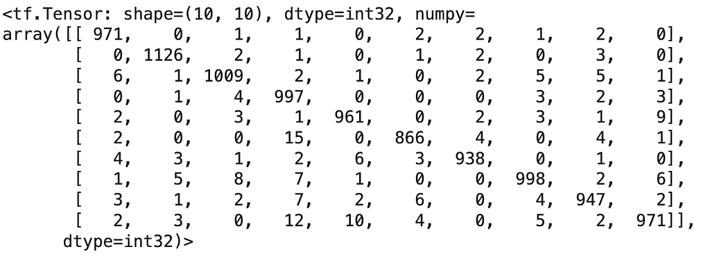
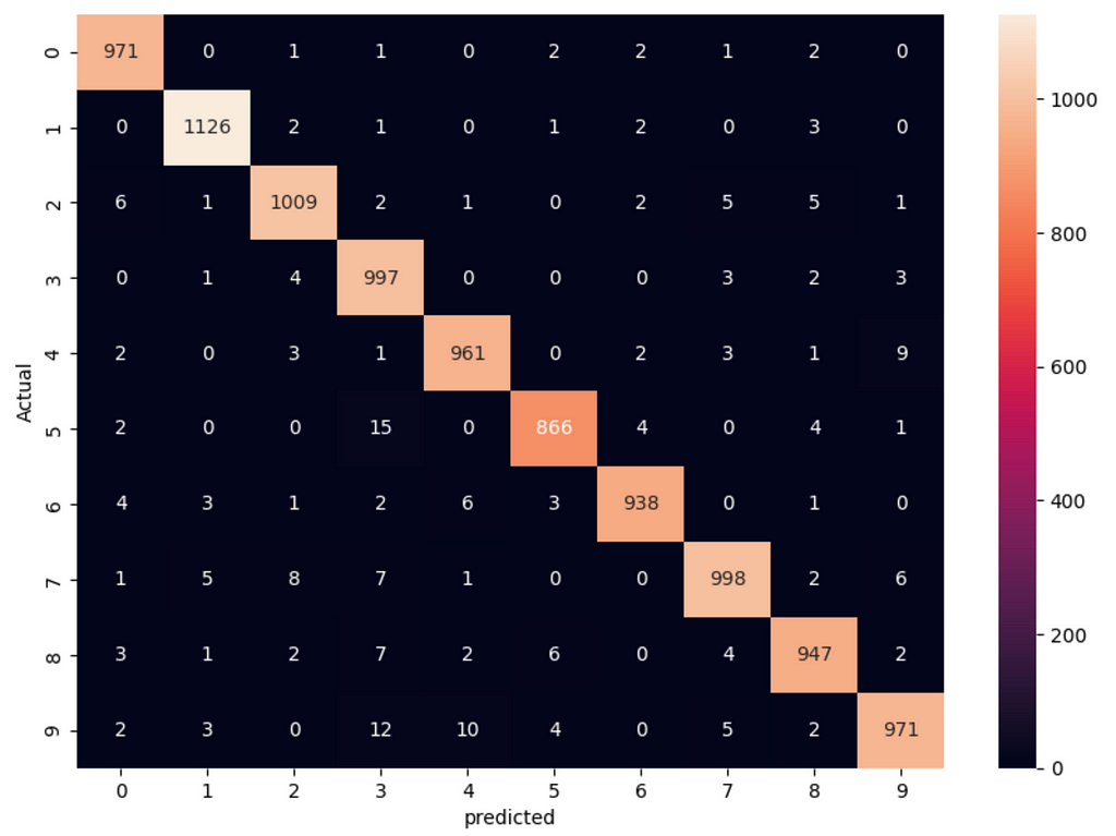
We then create the confusion matrix and visualize it.
cm = tf.math.confusion_matrix(labels=y_test, predictions=y_predicted_labels2)
plt.figure(figsize=(10, 7))
sns.heatmap(cm, annot=True, fmt='d')
plt.xlabel("Predicted")
plt.ylabel("Actual")
plt.show()
- tf.math.confusion_matrix(labels=y_test, predictions=y_predicted_labels2) generates the confusion matrix.
- sns.heatmap(cm, annot=True, fmt=’d’) visualizes the confusion matrix with annotations.
Conclusion
In this blog post, we covered the basics of deep learning and walked through the steps of building, training, and evaluating a simple ANN model using the MNIST dataset. We also improved the model by adding a hidden layer and using a different activation function. Deep learning models, though seemingly complex, can be built and understood step-by-step, enabling us to tackle various machine learning problems.
This brings us to the end of this article. I hope you have understood everything clearly. Make sure you practice as much as possible.
If you wish to check out more resources related to Data Science, Machine Learning and Deep Learning you can refer to my Github account.
You can connect with me on LinkedIn — RAVJOT SINGH.
I hope you like my article. From a future perspective, you can try other algorithms also, or choose different values of parameters to improve the accuracy even further. Please feel free to share your thoughts and ideas.
P.S. Claps and follows are highly appreciated.
Building Your First Deep Learning Model: A Step-by-Step Guide was originally published in Becoming Human: Artificial Intelligence Magazine on Medium, where people are continuing the conversation by highlighting and responding to this story.
3 Important Considerations in DDPG Reinforcement Algorithm

Deep Deterministic Policy Gradient (DDPG) is a Reinforcement learning algorithm for learning continuous actions. You can learn more about it in the video below on YouTube:
https://youtu.be/4jh32CvwKYw?si=FPX38GVQ-yKESQKU
Here are 3 important considerations you will have to work on while solving a problem with DDPG. Please note that this is not a How-to guide on DDPG but a what-to guide in the sense that it only talks about what areas you will have to look into.
Noise
Ornstein-Uhlenbeck
The original implementation/paper on DDPG mentioned using noise for exploration. It also suggested that the noise at a step depends on the noise in the earlier step. The implementation of this noise is the Ornstein-Uhlenbeck process. Some people later got rid of this constraint about the noise and just used random noise. Based on your problem domain, you may not be OK to keep noise at a step related to the noise at the earlier step. If you keep your noise at a step dependent on the noise at the earlier step, then your noise will be in one direction of the noise mean for some time and may limit the exploration. For the problem I am trying to solve with DDPG, a simple random noise works just fine.
Size of Noise
The size of noise you use for exploration is also important. If your valid action for your problem domain is from -0.01 to 0.01 there is not much benefit by using a noise with a mean of 0 and standard deviation of 0.2 as you will let your algorithm explore invalid areas using noise of higher values.
Noise decay
Many blogs talk about decaying the noise slowly during training, while many others do not and continue to use un-decayed during training. I think a well-trained algorithm will work fine with both options. If you do not decay the noise, you can just drop it during prediction, and a well-trained network and algorithm will be fine with that.
Soft update of the target networks
As you update your policy neural networks, at a certain frequency, you will have to pass a fraction of the learning to the target networks. So there are two aspects to look at here — At what frequency do you want to pass the learning (the original paper says after every update of the policy network) to the target networks and what fraction of the learning do you want to pass on to the target network? A hard update to the target networks is not recommended, as that destabilizes the neural network.
But a hard update to the target network worked fine for me. Here is my thought process — Say, your learning rate for the policy network is 0.001 and you update the target network with 0.01 of this every time you update your policy network. So in a way, you are passing 0.001*0.01 of the learning to the target network. If your neural network is stable with this, it will very well be stable if you do a hard update (pass all the learning from the policy network to the target network every time you update the policy network), but keep the learning rate very low.
Neural network design
While you are working on optimizing your DDPG algo parameters, you also need to design a good neural network for predicting action and value. This is where the challenge lies. It is difficult to tell if the bad performance of your solution is due to the bad design of the neural network or an unoptimized DDPG algo. You will need to keep optimizing on both fronts.
While a simpleton neural network can help you solve Open AI gym problems, it will not be sufficient for a real-world complex problem. The principle I follow while designing a neural network is that the neural network is an implementation of your (or the domain expert’s) mental framework of the solution. So you need to understand the mental framework of the domain expert in a very fundamental manner to implement it in a neural network. You also need to understand what features to pass to the neural network and how to engineer the features in a way that the neural network can interpret them to successfully predict. And that is where the art of the craft lies.
I still have not explored discount rate (which is used to discount rewards over time-steps) and have not yet developed a strong intuition (which is very important) about it.
I hope you liked the article and did not find it overly simplistic or stupid. If liked it, please do not forget to clap!
3 Important Considerations in DDPG Reinforcement Algorithm was originally published in Becoming Human: Artificial Intelligence Magazine on Medium, where people are continuing the conversation by highlighting and responding to this story.