Python has emerged as one of the most popular programming languages for machine learning due to its simplicity, flexibility, and robust ecosystem. As artificial intelligence (AI) and machine learning continue to transform industries, Python’s role in this domain is crucial, helping data scientists and engineers build models that are both powerful and scalable. Understanding why […]

The field of Natural Language Processing (NLP) has seen significant advancements in recent years, largely driven by the development of sophisticated models capable of understanding and generating human language. One of the key players in this revolution is Hugging Face, an open-source AI company that provides state-of-the-art models for a wide range of NLP tasks. Hugging Face’s Transformers library has become the go-to resource for developers and researchers looking to implement powerful NLP solutions.

Inbound-leads-automatically-with-ai. These models are trained on vast amounts of data and fine-tuned to achieve exceptional performance on specific tasks. The platform also provides tools and resources to help users fine-tune these models on their own datasets, making it highly versatile and user-friendly.

In this blog, we’ll delve into how to use the Hugging Face library to perform several NLP tasks. We’ll explore how to set up the environment, and then walk through examples of sentiment analysis, zero-shot classification, text generation, summarization, and translation. By the end of this blog, you’ll have a solid understanding of how to leverage Hugging Face models to tackle various NLP challenges.

Setting Up the Environment

First, we need to install the Hugging Face Transformers library, which provides access to a wide range of pre-trained models. You can install it using the following command:

!pip install transformers

This library simplifies the process of working with advanced NLP models, allowing you to focus on building your application rather than dealing with the complexities of model training and optimization.

Task 1: Sentiment Analysis

Sentiment analysis determines the emotional tone behind a body of text, identifying it as positive, negative, or neutral. Here’s how it’s done using Hugging Face:

from transformers import pipeline

classifier = pipeline("sentiment-analysis", token = access_token, model='distilbert-base-uncased-finetuned-sst-2-english')

classifier("This is by far the best product I have ever used; it exceeded all my expectations.")

In this example, we use the sentiment-analysis pipeline to classify the sentiments of sentences, determining whether they are positive or negative.

Task 2: Zero-Shot Classification

Zero-shot classification allows the model to classify text into categories without any prior training on those specific categories. Here’s an example:

classifier = pipeline("zero-shot-classification")
classifier(
    "Photosynthesis is the process by which green plants use sunlight to synthesize nutrients from carbon dioxide and water.",
    candidate_labels=["education", "science", "business"],
)

The zero-shot-classification pipeline classifies the given text into one of the provided labels. In this case, it correctly identifies the text as being related to “science”.

Task 3: Text Generation

In this task, we explore text generation using a pre-trained model. The code snippet below demonstrates how to generate text using the GPT-2 model:

generator = pipeline("text-generation", model="distilgpt2")

generator(

"Just finished an amazing book",

max_length=40, num_return_sequences=2,

)

Here, we use the pipeline function to create a text generation pipeline with the distilgpt2 model. We provide a prompt (“Just finished an amazing book”) and specify the maximum length of the generated text. The result is a continuation of the provided prompt.

Task 4: Text Summarization

Next, we use Hugging Face to summarize a long text. The following code shows how to summarize a piece of text using the BART model:

summarizer = pipeline("summarization")
text = """
San Francisco, officially the City and County of San Francisco, is a commercial and cultural center in the northern region of the U.S. state of California. San Francisco is the fourth most populous city in California and the 17th most populous in the United States, with 808,437 residents as of 2022.
"""
summary = summarizer(text, max_length=50, min_length=25, do_sample=False)
print(summary)

The summarization pipeline is used here, and we pass a lengthy piece of text about San Francisco. The model returns a concise summary of the input text.

Task 5: Translation

In the final task, we demonstrate how to translate text from one language to another. The code snippet below shows how to translate French text to English using the Helsinki-NLP model:

translator = pipeline("translation", model="Helsinki-NLP/opus-mt-fr-en")
translation = translator("L'engagement de l'entreprise envers l'innovation et l'excellence est véritablement inspirant.")
print(translation)

Here, we use the translation pipeline with the Helsinki-NLP/opus-mt-fr-en model. The French input text is translated into English, showcasing the model’s ability to understand and translate between languages.

Conclusion

The Hugging Face library offers powerful tools for a variety of NLP tasks. By using simple pipelines, we can perform sentiment analysis, zero-shot classification, text generation, summarization, and translation with just a few lines of code. This notebook serves as an excellent starting point for exploring the capabilities of Hugging Face models in NLP projects.

Feel free to experiment with different models and tasks to see the full potential of Hugging Face in action!

This brings us to the end of this article. I hope you have understood everything clearly. Make sure you practice as much as possible.

If you wish to check out more resources related to Data Science, Machine Learning, and Deep Learning, you can refer to my GitHub account.

You can connect with me on LinkedIn — Ravjot Singh.

P.S. Claps and follows are highly appreciated.

---

Unlocking the Power of Hugging Face for NLP Tasks was originally published in Becoming Human: Artificial Intelligence Magazine on Medium, where people are continuing the conversation by highlighting and responding to this story.

Are you curious about how different neural networks stack up against each other? In this blog, we dive into an exciting comparison between Artificial Neural Networks (ANN) and Convolutional Neural Networks (CNN) using the popular CIFAR-10 dataset. We’ll break down the key concepts, architectural differences, and real-world applications of ANNs and CNNs. Join us as we uncover which model reigns supreme for image classification tasks and why. Let’s get started!

Dataset Overview

The CIFAR-10 dataset is a widely-used dataset for machine learning and computer vision tasks. It consists of 60,000 32×32 color images in 10 different classes, with 50,000 training images and 10,000 test images. The classes are airplanes, cars, birds, cats, deer, dogs, frogs, horses, ships, and trucks. This blog explores the performance of Artificial Neural Networks (ANN) and Convolutional Neural Networks (CNN) on the CIFAR-10 dataset.

What is ANN?

Artificial Neural Networks (ANN) are computational models inspired by the human brain. They consist of interconnected groups of artificial neurons (nodes) that process information using a connectionist approach. ANNs are used for a variety of tasks, including classification, regression, and pattern recognition.

Principles of ANN

• Layers: ANNs consist of input, hidden, and output layers.
• Neurons: Each layer has multiple neurons that process inputs and produce outputs.
• Activation Functions: Functions like ReLU or Sigmoid introduce non-linearity, enabling the network to learn complex patterns.
• Backpropagation: The learning process involves adjusting weights based on the error gradient.

ANN Architecture

ANN = models.Sequential([
    layers.Flatten(input_shape=(32, 32, 3)),
    layers.Dense(3000, activation='relu'),
    layers.Dense(1000, activation='relu'),
    layers.Dense(10, activation='sigmoid')
])
ANN.compile(optimizer='adam', loss='sparse_categorical_crossentropy', metrics=['accuracy'

What is CNN?

Convolutional Neural Networks (CNN) are specialized ANNs designed for processing structured grid data, like images. They are particularly effective for tasks involving spatial hierarchies, such as image classification and object detection.

Principles of CNN

• Convolutional Layers: These layers apply convolutional filters to the input to extract features.
• Pooling Layers: Pooling layers reduce the spatial dimensions, retaining important information while reducing computational load.
• Fully Connected Layers: After convolutional and pooling layers, fully connected layers are used to make final predictions.

CNN Architecture

CNN = models.Sequential([
    layers.Conv2D(input_shape=(32, 32, 3), filters=32, kernel_size=(3, 3), activation='relu'),
    layers.MaxPooling2D((2, 2)),
    layers.Conv2D(filters=64, kernel_size=(3, 3), activation='relu'),
    layers.MaxPooling2D((2, 2)),
    layers.Flatten(),
    layers.Dense(2000, activation='relu'),
    layers.Dense(1000, activation='relu'),
    layers.Dense(10, activation='softmax')
])
CNN.compile(optimizer='adam', loss='sparse_categorical_crossentropy', metrics=['accuracy'])

Training and Evaluation

Both models were trained for 10 epochs on the CIFAR-10 dataset. The ANN model uses dense layers and is simpler, while the CNN model uses convolutional and pooling layers, making it more complex and suitable for image data.

ANN.fit(X_train, y_train, epochs=10)
ANN.evaluate(X_test, y_test)

CNN.fit(X_train, y_train, epochs=10)
CNN.evaluate(X_test, y_test)

Results Comparison

The evaluation results for both models show the accuracy and loss on the test data.

ANN Evaluation

• Accuracy: 0.4960
• Loss: 1.4678

CNN Evaluation

• Accuracy: 0.7032
• Loss: 0.8321

The CNN significantly outperforms the ANN in terms of accuracy and loss.

Confusion Matrices and Classification Reports

To further analyze the models’ performance, confusion matrices and classification reports were generated.

ANN Confusion Matrix and Report

y_pred_ann = ANN.predict(X_test)
y_pred_labels_ann = [np.argmax(i) for i in y_pred_ann]
plot_confusion_matrix(y_test, y_pred_labels_ann, "Confusion Matrix for ANN")
print("Classification Report for ANN:")
print(classification_report(y_test, y_pred_labels_ann))

CNN Confusion Matrix and Report

y_pred_cnn = CNN.predict(X_test)
y_pred_labels_cnn = [np.argmax(i) for i in y_pred_cnn]
plot_confusion_matrix(y_test, y_pred_labels_cnn, "Confusion Matrix for CNN")
print("Classification Report for CNN:")
print(classification_report(y_test, y_pred_labels_cnn))

Conclusion

The CNN model outperforms the ANN model on the CIFAR-10 dataset due to its ability to capture spatial hierarchies and local patterns in the image data. While ANNs are powerful for general tasks, CNNs are specifically designed for image-related tasks, making them more effective for this application.

In summary, for image classification tasks like those in the CIFAR-10 dataset, CNNs offer a significant performance advantage over ANNs due to their specialized architecture tailored for processing visual data.

This brings us to the end of this article. I hope you have understood everything clearly. Make sure you practice as much as possible.

If you wish to check out more resources related to Data Science, Machine Learning and Deep Learning you can refer to my Github account.

You can connect with me on LinkedIn — RAVJOT SINGH.

P.S. Claps and follows are highly appreciated.

---

Comparing ANN and CNN on CIFAR-10: A Comprehensive Analysis was originally published in Becoming Human: Artificial Intelligence Magazine on Medium, where people are continuing the conversation by highlighting and responding to this story.

Natural Language Processing (NLP) is a fascinating field that bridges the gap between human communication and machine understanding. One of the fundamental steps in NLP is text preprocessing, which transforms raw text data into a format that can be effectively analyzed and utilized by algorithms. In this blog, we’ll delve into three essential NLP preprocessing techniques: stopwords removal, bag of words, and word cloud generation. We’ll explore what each technique is, why it’s used, and how to implement it using Python. Let’s get started!

Stopwords Removal: Filtering Out the Noise

What Are Stopwords?

Stopwords are common words that carry little meaningful information and are often removed from text data during preprocessing. Examples include “the,” “is,” “in,” “and,” etc. Removing stopwords helps in focusing on the more significant words that contribute to the meaning of the text.

Why remove stopwords?

Stopwords are removed from:

• Reduce the dimensionality of the text data.
• Improve the efficiency and performance of NLP models.
• Enhance the relevance of features extracted from the text.

Pros and Cons

Pros:

• Simplifies the text data.
• Reduces computational complexity.
• Focuses on meaningful words.

Cons:

• Risk of removing words that may carry context-specific importance.
• Some NLP tasks may require stopwords for better understanding.

Implementation

Let’s see how we can remove stopwords using Python:

import nltk
from nltk.corpus import stopwords

# Download the stopwords dataset
nltk.download('stopwords')

# Sample text
text = "This is a simple example to demonstrate stopword removal in NLP."

Load the set of stopwords in English
stop_words = set(stopwords.words('english'))

Tokenize the text into individual words
words = text.split()

Remove stopwords from the text
filtered_text = [word for word in words if word.lower() is not in stop_words]

print("Original Text:", text)
print("Filtered Text:", " ".join(filtered_text))

Code Explanation

Importing Libraries:

import nltk from nltk.corpus import stopwords

We import thenltk library and the stopwords module fromnltk.corpus.

Downloading Stopwords:

nltk.download('stopwords')

This line downloads the stopwords dataset from the NLTK library, which includes a list of common stopwords for multiple languages.

Sample Text:

text = "This is a simple example to demonstrate stopword removal in NLP."

We define a sample text that we want to preprocess by removing stopwords.

Loading Stopwords:

stop_words = set(stopwords.words(‘english’))

We load the set of English stopwords into the variable stop_words.

Tokenizing Text:

words = text.split()

The split() method tokenizes the text into individual words.

Removing Stopwords:

filtered_text = [word for word in words if word.lower() is not in stop_words]

We use a list comprehension to filter out stopwords from the tokenized words. The lower() method ensures case insensitivity.

Printing Results:

print("Original Text:", text) print("Filtered Text:", ""). join(filtered_text))

Finally, we print the original text and the filtered text after removing stopwords.

Bag of Words: Representing Text Data as Vectors

What Is Bag of Words?

The Bag of Words (BoW) model is a technique to represent text data as vectors of word frequencies. Each document is represented as a vector where each dimension corresponds to a unique word in the corpus, and the value indicates the word’s frequency in the document.

Why Use Bag of Words?

bag of Words is used to:

• Convert text data into numerical format for machine learning algorithms.
• Capture the frequency of words, which can be useful for text classification and clustering tasks.

Pros and Cons

Pros:

• Simple and easy to implement.
• Effective for many text classification tasks.

Cons:

• Ignores word order and context.
• Can result in high-dimensional sparse vectors.

Implementation

Here’s how to implement the Bag of Words model using Python:

from sklearn.feature_extraction.text import CountVectorizer

# Sample documents
documents = [
    'This is the first document',
    'This document is the second document',
    'And this is the third document.',
    'Is this the first document?'
]

# Initialize CountVectorizer
vectorizer = CountVectorizer()

Fit and transform the documents
X = vectorizer.fit_transform(documents)

# Convert the result to an array
X_array = X.toarray()

# Get the feature names
feature_names = vectorizer.get_feature_names_out()

# Print the feature names and the Bag of Words representation
print("Feature Names:", feature_names)
print (Bag of Words: n", X_array)

Code Explanation

• Importing Libraries:

from sklearn.feature_extraction.text import CountVectorizer

We import the CountVectorizer from the sklearn.feature_extraction.text module.

Sample Documents:

documents = [ ‘This is the first document’, ‘This document is the second document’, ‘And this is the third document.’, ‘Is this is the first document?’ ]

We define a list of sample documents to be processed.

Initializing CountVectorizer:

vectorizer = CountVectorizer()

We create an instance ofCountVectorizer.

Fitting and Transforming:

X = vectorizer.fit_transform(documents)

Thefit_transform method is used to fit the model and transform the documents into a bag of words.

Converting to an array:

X_array = X.toarray()

We convert the sparse matrix result to a dense array for easy viewing.

Getting Feature Names:

feature_names = vectorizer.get_feature_names_out()

The get_feature_names_out method retrieves the unique words identified in the corpus.

Printing Results:

print(“Feature Names:”, feature_names) print(“Bag of Words: n”, X_array)

Finally, we print the feature names and the bag of words.

Word Cloud: Visualizing Text Data

What Is a Word Cloud?

A word cloud is a visual representation of text data where the size of each word indicates its frequency or importance. It provides an intuitive and appealing way to understand the most prominent words in a text corpus.

Why Use Word Cloud?

Word clouds are used to:

• Quickly grasp the most frequent terms in a text.
• Visually highlight important keywords.
• Present text data in a more engaging format.

Pros and Cons

Pros:

• Easy to interpret and visually appealing.
• Highlights key terms effectively.

Cons:

• Can oversimplify the text data.
• May not be suitable for detailed analysis.

Implementation

Here’s how to create a word cloud using Python:

from wordcloud import WordCloud
import matplotlib.pyplot as plt

# Sample text
df = pd.read_csv('/content/AmazonReview.csv')

comment_words = ""

stopwords = set(STOPWORDS)

for val in df.Review:
     val = str(val)
     tokens = val.split()
     for i in range(len(tokens)):
     tokens[i] = tokens[i].lower()
     comment_words += "".join(tokens) + ""

pic = np.array(Image.open(requests.get('https://www.clker.com/cliparts/a/c/3/6/11949855611947336549home14.svg.med.png', stream = True).raw))

# Generate word clouds
wordcloud = WordCloud(width=800, height=800, background_color='white', mask=pic, min_font_size=12).generate(comment_words)

Display the word cloud
plt.figure(figsize=(8,8), facecolor=None)
plt.imshow(wordcloud)
plt.axis('off')
plt.tight_layout(pad=0)
plt.show()

Code Explanation

• Importing Libraries:

from wordcloud import WordCloud import matplotlib.pyplot as plt

We import the WordCloud class from the wordcloud library and matplotlib.pyplot for displaying the word cloud.

Generating Word Clouds:

wordcloud = WordCloud(width=800, height=800, background_color=’white’).generate(comment_words)

We create an instance of WordCloud with specified dimensions and background color and generate the word cloud using the sample text.

Conclusion

In this blog, we’ve explored three essential NLP preprocessing techniques: stopwords removal, bag of words, and word cloud generation. Each technique serves a unique purpose in the text preprocessing pipeline, contributing to the overall effectiveness of NLP tasks. By understanding and implementing these techniques, we can transform raw text data into meaningful insights and powerful features for machine learning models. Happy coding and exploring the world of NLP!

This brings us to the end of this article. I hope you have understood everything clearly. Make sure you practice as much as possible.

If you wish to check out more resources related to Data Science, Machine Learning and Deep learning, you can refer to my Github account.

You can connect with me on LinkedIn — RAVJOT SINGH.

I hope you like my article. From a future perspective, you can try other algorithms or choose different values of parameters to improve the accuracy even further. Please feel free to share your thoughts and ideas.

P.S. Claps and follows are highly appreciated.

---

Exploring NLP Preprocessing Techniques: Stopwords, Bag of Words, and Word Cloud was originally published in Becoming Human: Artificial Intelligence Magazine on Medium, where people are continuing the conversation by highlighting and responding to this story.

Welcome, Firebase enthusiasts!

Today, we’re venturing into the realm of serverless computing that can be integrated with AI using Python language to explore the wonders of cloud functions with Python, specifically with Firebase Cloud Functions. These functions offer a seamless way to execute code in response to various triggers, all without the hassle of managing servers.

But before we dive deep into serverless territory, let’s briefly compare this approach with another popular architectural pattern: microservices.

Serverless Cloud Functions vs. Microservices

Serverless cloud functions and microservices are both architectural patterns used to build scalable and flexible applications. However, they differ in several key aspects:

1. Resource Management:

• Serverless Cloud Functions: With serverless functions, cloud providers handle infrastructure management, including server provisioning, scaling, and maintenance. Developers focus solely on writing code without worrying about underlying infrastructure.
• Microservices: Microservices require developers to manage their own infrastructure, including servers, containers, and orchestration tools like Kubernetes. While this offers more control over resources, it also adds complexity and overhead.

2. Scaling:

• Serverless Cloud Functions: Cloud functions automatically scale up or down based on demand. Providers allocate resources dynamically, ensuring optimal performance and cost efficiency.
• Microservices: Scaling microservices involves manual or automated management of resources. Developers must anticipate traffic patterns and adjust resource allocation accordingly, which can be challenging to implement and maintain at scale.

3. Cost:

• Serverless Cloud Functions: Serverless functions offer a pay-as-you-go pricing model, where you’re charged only for the resources used during execution. This can be cost-effective for sporadic workloads with unpredictable traffic.
• Microservices: Microservices require constant resource allocation, regardless of workload fluctuations. While this provides more predictable costs, it can lead to overprovisioning and wasted resources during periods of low activity.

4. Development and Deployment:

• Serverless Cloud Functions: Developing and deploying serverless functions is straightforward and requires minimal setup. Developers focus on writing code, and deployment is handled through simple CLI commands or CI/CD pipelines.
• Microservices: Developing and deploying microservices involves more upfront setup, including infrastructure provisioning, containerization, and service discovery. Managing dependencies and versioning across multiple services adds complexity to the development and deployment process.

Now that we’ve outlined the differences between serverless cloud functions and microservices, let’s delve into the specifics of building and deploying cloud functions with Python using Firebase Cloud Functions.

Without further ado, let’s get started by setting up our Firebase project.

Step 1: Set Up Your Firebase Project

Ensure you have Python installed on your system. If you haven’t already, install the Firebase CLI globally using npm:

npm install -g firebase-tools

Next, log in to your Google account and initialize a Firebase project in your desired directory. During the initialization process.

firebase login
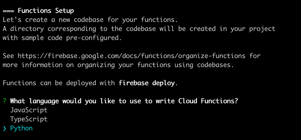
firebase init functions

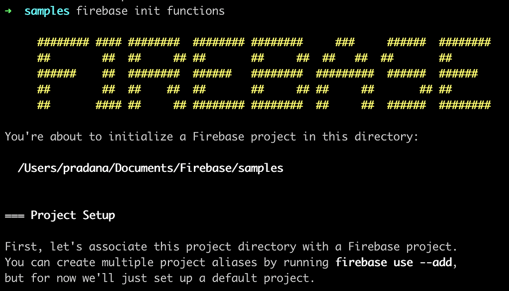
you’ll be prompted to choose either JavaScript or TypeScript as your default language. Select Python if prompted.

After that, you will be given this project structure to get started with!

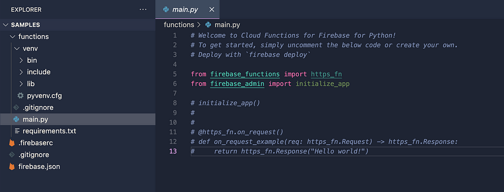
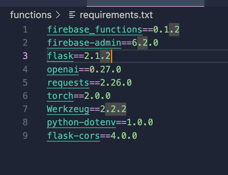
Now, before we proceed to the code, do not forget to add Flask into the requirements.txt to integrate Flask into our Cloud Functions, at the time of writing I do recommend using version 2.1.2 for the supported version with Cloud Functions.

Then let’s install all necessary dependencies with

python -m venv functions/venv
source functions/venv/bin/activate && python -m pip install -r functions/requirements.txt

Step 2: Write Your Python Function

Now, let’s write some Python code for our cloud function. For this example, let’s create a simple function that responds to HTTP requests with a friendly greeting.

Navigate to the functions directory created by the Firebase CLI and open the main.py file. Replace the contents with the following Python code:

from firebase_functions import https_fn
from flask import Flask

app = Flask(__name__)

@app.route('/')
def hello_world():
    return 'Hello, Firebase Cloud Functions with Python'

@https_fn.on_request(max_instances=1)
def articles(req: https_fn.Request) -> https_fn.Response:
    with app.request_context(req.environ):
        return app.full_dispatch_request()

The code above will wrap your Flask python framework inside the Firebase Cloud Functions. which means

“ 1 Cloud Function can wrap multiple Flask API Endpoints”

For an example, we have a cloud functions named “articles” where we can have several API endpoints such as
– /contents
– /images
– /generators etc.
I other words, you can also treat a Cloud Functions stand as a Microservice, where they had their own responsibility for the scope and contents.

Step 3: Deploy Your Cloud Function

With our function ready, it’s time to deploy it to Firebase. Run the following command from your project directory to deploy your function

firebase deploy --only functions

Step 4: Test Your Cloud Function

Once deployed, you can test your cloud function by sending an HTTP request to its trigger URL. You can find the URL in the Firebase console under the “Functions” tab.

Now, open your favorite browser or use a tool like cURL to send a GET request to the trigger URL. You should receive a friendly greeting in response!

curl https://YOUR_CLOUD_FUNCTION_ID.run.app/YOUR_API_NAME

Congratulations! You’ve successfully built and deployed your first cloud function with Python using Firebase Cloud Functions.

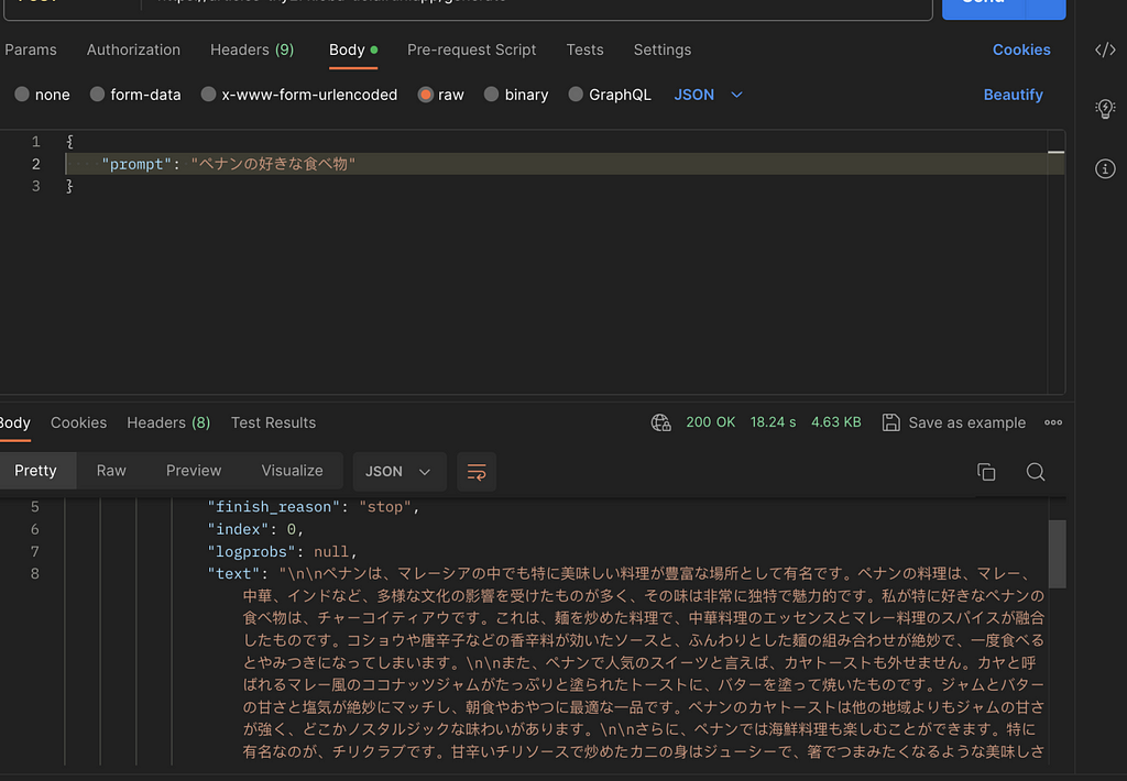
Now you can hit your deployed cloud functions through Postman as well which in my case I have a POST API called /generate to generate articles with Generative AI. I will share more about this in another article!

So, In summary, we have learned :
– Understand the benefit of using serverless over microservice
– Setup Firebase Cloud Functions using Python
– Integrate Flask into our Python Firebase Cloud Functions.
– Deploy our Flask Firebase Cloud Functions

If you need the source code feel free to fork it from here : https://github.com/retzd-tech/genai-openai-firebase-function-sample

That’s it!

If you are up for next level, you can implement a more intelligent AI LLM Model, feel free to read it here!

whether you’re building a Generative AI Application, web application, processing data, or automating tasks, Firebase Cloud Functions with Python have got you covered. Happy coding in the cloud!

---

Future AI backend processing : Leveraging Flask Python on Firebase Cloud Functions was originally published in Becoming Human: Artificial Intelligence Magazine on Medium, where people are continuing the conversation by highlighting and responding to this story.

Python has remained one of the most popular programming languages in software development since its inception in 1991. Python is fairly well known for its web development capabilities. However, one of the biggest strengths of Python is its ability to adapt to new requirements and technologies. The biggest evidence of its adaptability and versatility to […]

Your meeting minutes generated automatically in a document with ChatGPT right after recording your meeting

1. Unleash the Power of ChatGPT to Do (Useful) Things

In this technical article, we will explore how to leverage the ChatGPT 4 API along with Google Meet, Google Drive, and Google Docs APIs to automatically generate meeting minutes.

Taking minutes during a meeting can be a time-consuming task, and it is often difficult to capture everything that is discussed. With the use of artificial intelligence, the process can be streamlined to ensure that nothing is missed.

As Microsoft Teams or Zoom, Google Meet has the ability to record meetings. Once the recording is activated, the transcript of the meeting is generated in a Google Document format and is stored on a defined Google Drive shared folder. Google Meet transcript file is used here but similar transcript text extract could also be done with Teams or Zoom recording.

For this, a simple web application will be used as a central point to manage the user interaction as well as the different API calls. The purpose is to display a list of these meeting transcript documents stored on a predefined Google Drive folder. The user will be able to select one of them then press a button to generate a summary of the meeting minutes as well as the action items with due dates. Also, these two new sections will be inserted in the same Google Document with Google Docs API, containing the results from ChatGPT API.

This article will walk you through the steps required to set up the necessary configuration and to understand the Dash/Python application code used to manage the ChatGPT, Google Drive & Docs APIs.

A link to my GitLab containing the full Python/Dash source code is also available on the next sections.

By the end of this article, I’ll also share my thoughts on some limitations and improvements that could be done on this application. I hope it will allow you to find new ideas on how to stay focused on more valuable tasks than taking meeting minutes.

So let’s dive in!

2. Overview of the web application capabilities

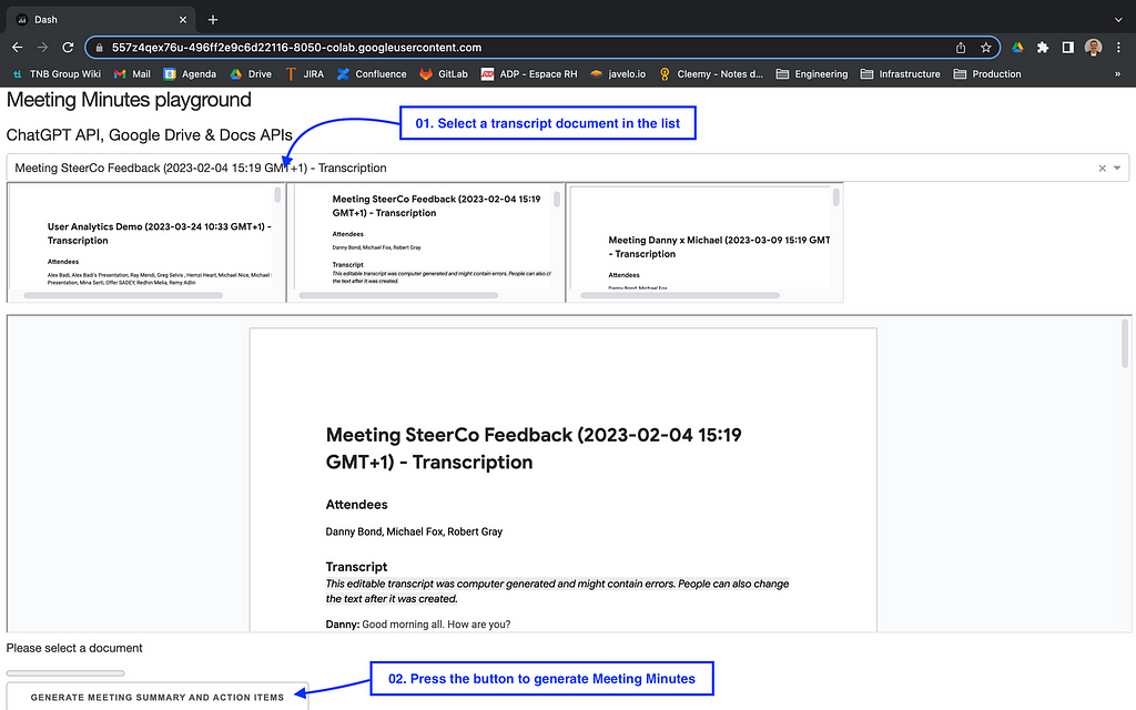
The web application looks like the screen below. The upper section displays a list of transcript documents present on the user’s shared Google Drive folder. Such documents are automatically generated in the ‘Meet Recordings’ folder when the user triggers the Google Meet recording button.

The user can select a document in the list. The selected document is displayed in the central part. Finally, the user can press the button to generate the meeting minutes.

Once the button pressed, the Meeting minutes are automatically inserted in 2 new sections:

The ‘Meeting Summary’ section is a short description of the meeting based on the meeting transcript. It will stay synthetic whatever the duration of the meeting.

The ‘Meeting Action Items’ section is a numbered action items checkbox list which is also based on the transcript. When known, a due date is also inserted.

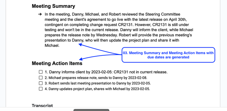
Each numbered meeting action item contains a checkbox that is natively supported by Google Docs. They could be used later on by your teams to follow up the action list and to check them once they are done.

3. Quick Start

The following will allow you to edit and run the code present on my GitLab. Before doing that, you’ll need to register at OpenAI to get your API key. Also, Google Drive and Docs APIs need to be activated on the Google console, as well as creating a Google Service Account.

• Go to the OpenAI website and sign up to get your API Key
• Go to my GitLab project named Meeting Minutes generation with ChatGPT
• Edit the Jupyter Python notebook with Google Colab and save it on your own Colab folder
• Replace the ‘OPENAI_API_KEY’ value in the code with your own api key
• Use the following link to activate the Google Drive & the Google Doc APIs
• Use the following link to create a Google Service Account
• Download and save the Google Service Account Key (JSon File) in your Colab folder. Name it ‘credentials_serviceaccount.json’ (or change the value in the code)
• Share your ‘Meet Recordings’ Google Drive folder with the Google Service Account created previously (with ‘Editor’ permission)
• Attend a Google Meet meeting. Record it with the transcript. The video file and the transcript document will automatically be generated in your ‘Meet Recordings’ Google Drive folder
• In the code, replace the ‘GOOGLE_MEET_RECORDING_FOLDER’ value with the ID of your ‘Meet Recordings’ Google Drive folder shared previously
• Select ‘Run All’ in the ‘Execution’ menu
• A WebApp should start in a few seconds. Click on the URL generated in the bottom of the Colab notebook to display it

The application should look like the first screenshot in the previous section.

4. Understand the main parts of the code

As of today, the ChatGPT 4 API is still in beta. The used version in the code is ‘gpt-4–0314’ snapshot. It can also be switched to the current version, ‘gpt-3.5-turbo’.

I’ll focus only on the most important pieces of the code.

4.1. Google Drive integration / API

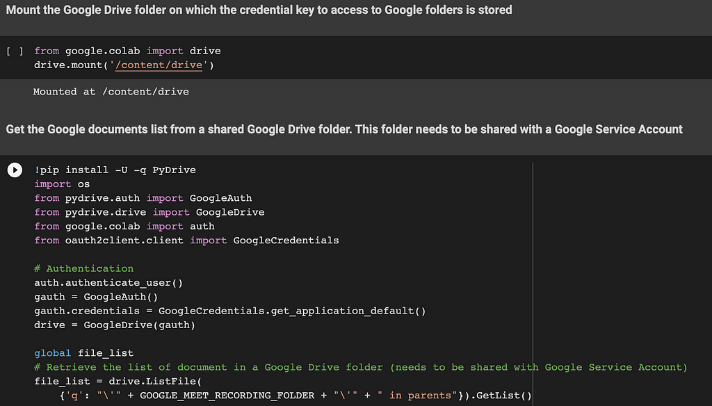
The first two lines of code are used to mount your Google Drive root folder. The main usage is to retrieve the Google Service Account credential key (JSon file) generated within the Quick Start section.

The code of the next section retrieves a file list of all transcript documents stored in the Google Meet Recording folder. The list will be used later to display these documents on the web application.

4.2. Google Meet transcript document text extract

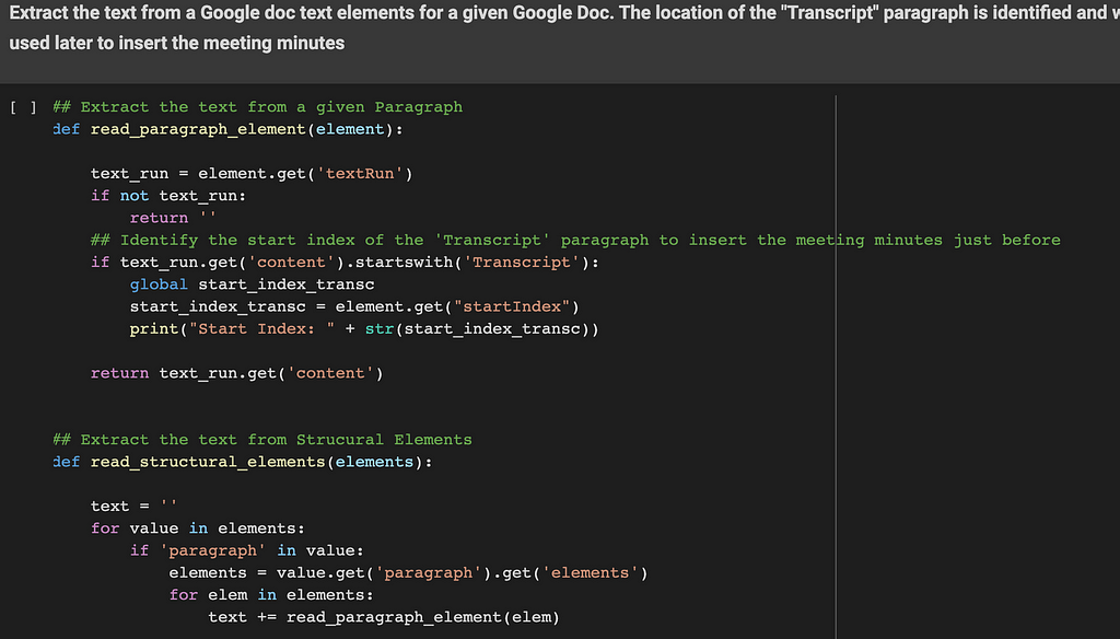
These functions are used to extract text elements from a defined Google Document ID. Google Meet generates a paragraph named ‘Transcript’. The location of the ‘Transcript’ section is identified and will be used later as a starting point to insert the meeting minutes. The two sections inserted by the application will be located just before this ‘Transcript’ section. (and right after the ‘Attendees’ section)

4.3. ChatGPT preparation: break down of the transcript text into chunks

ChatGPT API models have a limited number of tokens per request. In order to stay compatible with the ‘gpt-3.5-turbo’ model, the max value used in the code is 4096 tokens per request. But keep in mind that the ‘gpt-4’ model can handle much more. A 8k or a 32k models are also available, they can be used to significantly improve the meeting minutes’ quality for long meetings.

As a consequence, the Google Meet Transcript document text needs to be broken down into chunks of 4000 tokens with an overlap of 100 tokens.

These functions will prepare and return a list of chunks that will be used later by the ChatGPT API.

4.4. ChatGPT API usage

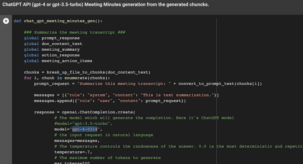
This function generates the meeting summary and action items in a few steps. A ChatGPT API call is done for each of them:

• Step 1: Summarize the meeting transcript text. The function iterates over the chunk list generated previously. The content sent to ChatGPT is based on the recorded conversation between the attendees. The ChatGPT API is called for each chunk with the following request: ‘Summarize this meeting transcript: <chunk>’
• Step 2: Consolidate the response (Meeting summary) from Step 1. The ChatGPT API is called with the following request: ‘Consolidate these meeting summaries: <ChatGPT responses from Step 1>’
• Step 3: Get action items with due dates from the transcript. The function iterates over the chunk list generated previously. The ChatGPT API is called for each chunk with the following request: ‘Provide a list of action items with a due date from the provided meeting transcript text: <chunk>’
• Step 4: Consolidate the meeting action items from Step 3 in a concise numbered list. The ChatGPT API is called with the following request: ‘Consolidate these meeting action items with a concise numbered list: <ChatGPT responses from Step 3>’

Each ChatGPT API used parameter (i.e. ‘temperature’) is documented in the code.

4.5. Google Docs API management usage to insert the final meeting minutes

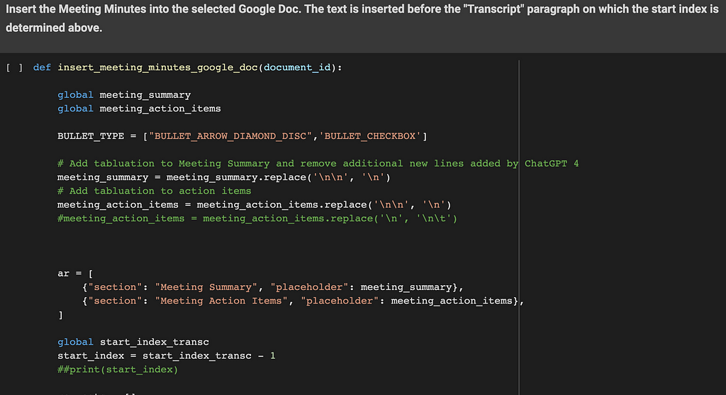
The objective of this function is to insert the meeting minutes into the Google Doc selected by the user. The text is inserted before the ‘Transcript’ paragraph. The start index identified in the previous functions is used here as a starting point.

Two sections are inserted here: ‘Meeting Summary’ and ‘Meeting Action items’.

Each section’s insertion is done with the following steps:

• the section’s title is inserted (as a text i.e. ‘Meeting Summary’)
• its style is set to ‘HEADING_1’, its text style is set to ‘bold’, its font size is set to ‘14’
• the section’s content is inserted (this comes from the ChatGPT API result)
• its style is set to ‘NORMAL’. A bullet point is also inserted with an arrow for the ‘Meeting Summary’ section and a checkbox for the ‘Meeting Action items’ section

Some ‘tabulation’ and ‘new line’ characters are also inserted to correct the text returned from the ChatGPT API.

Tip: Please note that the ‘ar’ table is iterated in a reversed way to ensure the start index position stays always up to date following each text insertion.

4.6. The main Python Dash Web Application

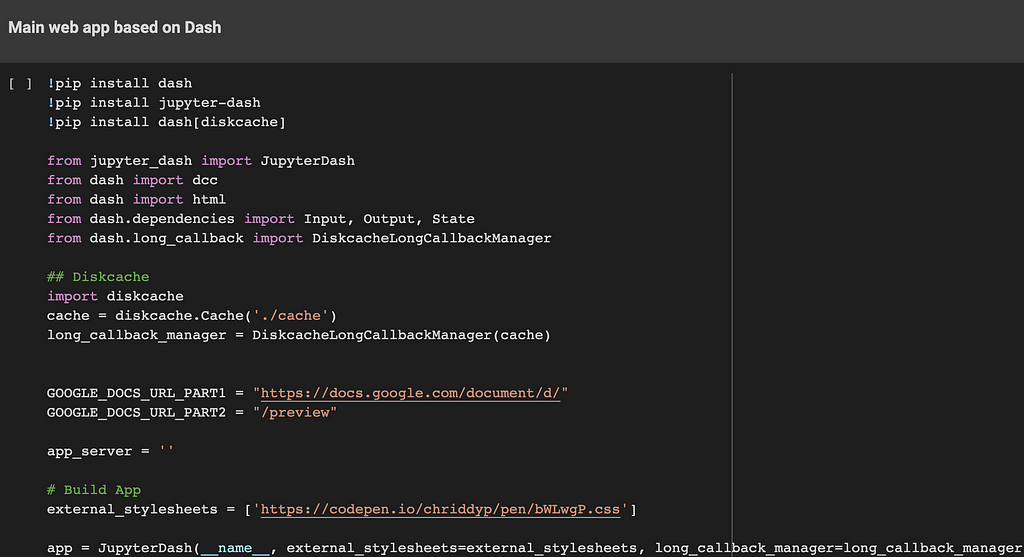
This part is used to build a simple web application on which the user can interact. Basically, it displays a list of documents stored on a Google Drive shared folder. The user can select one of them which is displayed in the central part of the screen. Once the button is pressed, the meeting minutes are inserted into this document. The updated document is refreshed with the results.

This code is built on top of the Dash framework. It even works within a Google Colab notebook.

Each document is displayed within a dedicated iFrame. The document’s link is based on ‘embedLink’ value, previously retrieved by the Google Drive API.

Also, a progress bar is displayed during the ChatGPT API calls and the Google Doc meeting minutes’ insertion steps.

5. Possible improvements

The main challenge using ChatGPT within your company is to have a leak of sensitive information your company is working on. This happened recently at Samsung where employees have accidentally leaked company secrets with ChatGPT.

One of the improvements of this code could be the execution of data masking before calling the ChatGPT API. At least the attendee names and additional tagged fields containing sensitive information should be masked. The meeting name could also contain some tags for data masking. I.e ‘Meeting with <Microsoft>’ where ‘Microsoft’ will be masked on the entire transcript document data extract. Once the response is received from ChatGPT API, the reverse needs to be done. Each masked information needs to be unmasked before calling the Google Docs API.

For this, a reference table needs to be used to store each field ID with its clear and its masked value. So these fields could be masked before calling the ChatGPT API, then unmasked when inserting the meeting minutes’ sections with Google Docs API.

6. The Final Word

Thank you for reading my article to the end, hope you enjoyed it!

As you can see, ChatGPT 4 API combined with Google Drive/Docs APIs are very powerful and can contribute significantly to improving your day-to-day work.

You can find the entire source code on my GitLab: Meeting Minutes generation with ChatGPT

---

Meeting minutes generation with ChatGPT 4 API, Google Meet, Google Drive & Docs APIs was originally published in Becoming Human: Artificial Intelligence Magazine on Medium, where people are continuing the conversation by highlighting and responding to this story.